Basic Tutorial for Toad
Toad is developed to facilitate the model development of credit risk scorecard particularly. In this tutorial, the basic use of toad will be introduced.
The tutorial will follow the common procedure of credit risk scorecard model development:
(1) EDA
(2) Feature selection and WOE binning
(3) Model selection
(4) Model validation
(5) Scorecard transformation
0. Data preparation
The data used is the famous german credit dataset. The following data preprocessing include:
- replacing target as 0, 1 from ‘good’ / ‘bad’;
- train test split;
and (3) adding a feature to indicate train and test. The training set will be used for modelling and the test set will only be used for validation
[1]:
'''
! Make sure to upgrade to the latest version !
'''
#!pip install --upgrade toad
[1]:
'\n! Make sure to upgrade to the latest version !\n'
[2]:
import pandas as pd
import numpy as np
from sklearn.linear_model import LogisticRegression
from sklearn.model_selection import train_test_split

import toad
[3]:
data = pd.read_csv('germancredit.csv')
data.replace({'good':0,'bad':1},inplace=True) # replace target as 0, 1.

print(data.shape) # 1000 data and 20 features
data.head()
(1000, 21)
[3]:
| status.of.existing.checking.account | duration.in.month | credit.history | purpose | credit.amount | savings.account.and.bonds | present.employment.since | installment.rate.in.percentage.of.disposable.income | personal.status.and.sex | other.debtors.or.guarantors | ... | property | age.in.years | other.installment.plans | housing | number.of.existing.credits.at.this.bank | job | number.of.people.being.liable.to.provide.maintenance.for | telephone | foreign.worker | creditability | |
|---|---|---|---|---|---|---|---|---|---|---|---|---|---|---|---|---|---|---|---|---|---|
| 0 | ... < 0 DM | 6 | critical account/ other credits existing (not ... | radio/television | 1169 | unknown/ no savings account | ... >= 7 years | 4 | male : single | none | ... | real estate | 67 | none | own | 2 | skilled employee / official | 1 | yes, registered under the customers name | yes | 0 |
| 1 | 0 <= ... < 200 DM | 48 | existing credits paid back duly till now | radio/television | 5951 | ... < 100 DM | 1 <= ... < 4 years | 2 | female : divorced/separated/married | none | ... | real estate | 22 | none | own | 1 | skilled employee / official | 1 | none | yes | 1 |
| 2 | no checking account | 12 | critical account/ other credits existing (not ... | education | 2096 | ... < 100 DM | 4 <= ... < 7 years | 2 | male : single | none | ... | real estate | 49 | none | own | 1 | unskilled - resident | 2 | none | yes | 0 |
| 3 | ... < 0 DM | 42 | existing credits paid back duly till now | furniture/equipment | 7882 | ... < 100 DM | 4 <= ... < 7 years | 2 | male : single | guarantor | ... | building society savings agreement/ life insur... | 45 | none | for free | 1 | skilled employee / official | 2 | none | yes | 0 |
| 4 | ... < 0 DM | 24 | delay in paying off in the past | car (new) | 4870 | ... < 100 DM | 1 <= ... < 4 years | 3 | male : single | none | ... | unknown / no property | 53 | none | for free | 2 | skilled employee / official | 2 | none | yes | 1 |
5 rows × 21 columns
[4]:
Xtr,Xts,Ytr,Yts = train_test_split(data.drop('creditability',axis=1),data['creditability'],test_size=0.25,random_state=450)
data_tr = pd.concat([Xtr,Ytr],axis=1)
data_tr['type'] = 'train' # A new feature to indicate test/training sample
data_ts = pd.concat([Xts,Yts],axis=1)
data_ts['type'] = 'test'

# The training set will be used for modelling and the test set will only be used for validation.

print(data_tr.shape)
#print(data_tr.head())
(750, 22)
| ___ |
|---|
| ### I. EDA data handling |
| Toad supports general EDA of each feature to detect missing values and feature distribution. |
- toad.detector.detect(): return the EDA report of each feature, incl. data type, distribution, missing rate, and unique values. The EDA report is aimed to guide missing / extreme value detection & replacing.
[5]:
toad.detector.detect(data_tr).head(10)
[5]:
| type | size | missing | unique | mean_or_top1 | std_or_top2 | min_or_top3 | 1%_or_top4 | 10%_or_top5 | 50%_or_bottom5 | 75%_or_bottom4 | 90%_or_bottom3 | 99%_or_bottom2 | max_or_bottom1 | |
|---|---|---|---|---|---|---|---|---|---|---|---|---|---|---|
| status.of.existing.checking.account | object | 750 | 0.00% | 4 | no checking account:39.20% | ... < 0 DM:27.60% | 0 <= ... < 200 DM:27.07% | ... >= 200 DM / salary assignments for at leas... | None | None | no checking account:39.20% | ... < 0 DM:27.60% | 0 <= ... < 200 DM:27.07% | ... >= 200 DM / salary assignments for at leas... |
| duration.in.month | int64 | 750 | 0.00% | 32 | 20.548 | 11.941 | 4 | 6 | 8 | 18 | 24 | 36 | 60 | 72 |
| credit.history | object | 750 | 0.00% | 5 | existing credits paid back duly till now:53.73% | critical account/ other credits existing (not ... | delay in paying off in the past:8.00% | all credits at this bank paid back duly:4.93% | no credits taken/ all credits paid back duly:3... | existing credits paid back duly till now:53.73% | critical account/ other credits existing (not ... | delay in paying off in the past:8.00% | all credits at this bank paid back duly:4.93% | no credits taken/ all credits paid back duly:3... |
| purpose | object | 750 | 0.00% | 10 | radio/television:27.47% | car (new):25.33% | furniture/equipment:18.40% | business:9.33% | car (used):9.20% | education:5.07% | repairs:2.67% | domestic appliances:1.07% | others:0.93% | retraining:0.53% |
| credit.amount | int64 | 750 | 0.00% | 700 | 3207.35 | 2731.93 | 250 | 417.33 | 906.3 | 2301.5 | 3956.5 | 7179.4 | 12715.2 | 15672 |
| savings.account.and.bonds | object | 750 | 0.00% | 5 | ... < 100 DM:60.93% | unknown/ no savings account:17.47% | 100 <= ... < 500 DM:10.53% | 500 <= ... < 1000 DM:6.00% | ... >= 1000 DM:5.07% | ... < 100 DM:60.93% | unknown/ no savings account:17.47% | 100 <= ... < 500 DM:10.53% | 500 <= ... < 1000 DM:6.00% | ... >= 1000 DM:5.07% |
| present.employment.since | object | 750 | 0.00% | 5 | 1 <= ... < 4 years:32.53% | ... >= 7 years:24.93% | ... < 1 year:18.67% | 4 <= ... < 7 years:17.60% | unemployed:6.27% | 1 <= ... < 4 years:32.53% | ... >= 7 years:24.93% | ... < 1 year:18.67% | 4 <= ... < 7 years:17.60% | unemployed:6.27% |
| installment.rate.in.percentage.of.disposable.income | int64 | 750 | 0.00% | 4 | 2.94533 | 1.13493 | 1 | 1 | 1 | 3 | 4 | 4 | 4 | 4 |
| personal.status.and.sex | object | 750 | 0.00% | 3 | male : single:54.40% | female : divorced/separated/married:36.27% | male : married/widowed:9.33% | None | None | None | None | male : single:54.40% | female : divorced/separated/married:36.27% | male : married/widowed:9.33% |
| other.debtors.or.guarantors | object | 750 | 0.00% | 3 | none:90.80% | guarantor:4.93% | co-applicant:4.27% | None | None | None | None | none:90.80% | guarantor:4.93% | co-applicant:4.27% |
II. Feature selection, fine classing, and WOE transformation
Toad can be used to filter abundant features such as the ones with high missing rate, low iv, and highly correlated features. It can also fine class features with vairous binning techniques and apply WOE transformation.
- toad.selection.select(): used to filter features based on missing percentage, iv (with 20 bins), and multicolleanrity (with VIF and/or intercorrelation)
[6]:
# The filter criteria include missing rate >=0.5, iv <= 0.05, correlation >= 0.7 (the one with the hightest iv will be kept),
# and "exclude = ['type']" specifies that 'type' tag will be not dropped
selected_data, drop_lst= toad.selection.select(data_tr,target = 'creditability', empty = 0.5, iv = 0.05, corr = 0.7, return_drop=True, exclude=['type'])

selected_test = data_ts[selected_data.columns]

print(selected_data.shape)
drop_lst # As shown, 8 features have been dropped due to low iv.
(750, 16)
[6]:
{'empty': array([], dtype=float64),
 'iv': array(['installment.rate.in.percentage.of.disposable.income',
        'present.residence.since',
        'number.of.existing.credits.at.this.bank', 'job',
        'number.of.people.being.liable.to.provide.maintenance.for',
        'telephone'], dtype=object),
 'corr': array([], dtype=object)}
- toad.quality(dataframe, target): return the quality of each feature, incl. iv, gini, and entropy. The output provides information of which features are potentially more useful.
[7]:
quality = toad.quality(data,'creditability')
quality.head(6)
[7]:
| iv | gini | entropy | unique | |
|---|---|---|---|---|
| status.of.existing.checking.account | 0.666012 | 0.368037 | 0.545196 | 4.0 |
| duration.in.month | 0.354784 | 0.406755 | 0.609659 | 33.0 |
| credit.amount | 0.351455 | 0.408680 | 0.610864 | 921.0 |
| credit.history | 0.293234 | 0.394090 | 0.580631 | 5.0 |
| age.in.years | 0.211197 | 0.414339 | 0.610863 | 53.0 |
| savings.account.and.bonds | 0.196010 | 0.404838 | 0.591377 | 5.0 |
__________
First, Combiner() to bin and set bins
- toad.transform.Combiner(): combiner is used to fine class numerical and categorical features with binning. We support Chi-squared binning, decision tree binning, binning by step, and binning by quantile. The following demonstrates the procedure.
3.1. combiner().fit(data, y = ‘target’, method = ‘chi’, min_samples = None, n_bins = None** )**: fit binning. Method supports ‘chi’, ‘dt’, ‘percentile’, and ‘step’.
3.2. combiner().set_rules(dict): used to set bins.
3.3. combiner().transform(data): transform the features of data into binned groups. ____ Second, WOETransformer() to WOE transform
- toad.transform.WOETransformer(): apply WOE transformation after binnning
4.1 WOETransformer().fit_transform(data, y_true, exclude = None): WOE transform data by data. “exclude” excludes the columns not to be transformed
4.2 WOETransformer().transform(data): transform data after fit_transform. Normally applied to test/validation data after fit_transform(training).
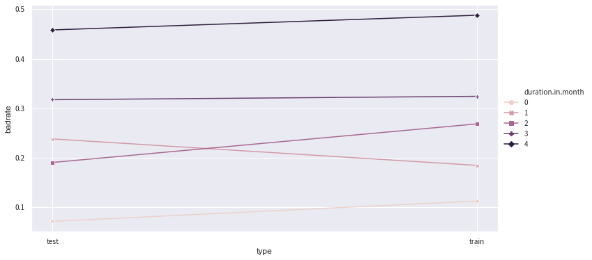
Use plots to tune bins.
- toad.plot.badrate_plot(data,target = ‘target’, x = None, by = None): plot the bad rate of each bin across different sets. Different sets can be train/test, or different month etc. “by” is name of the column to plot. “x” is the column used for comparison (e.g.month, test/train).
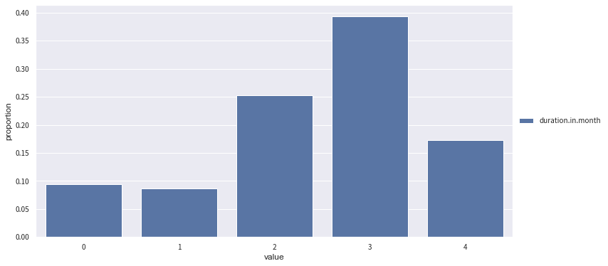
- toad.plot.proportion_plot(data[col]): plot the proportion each bin of a binned feature.
Note: the guide below is the binning as a whole, please refer to the `complete tutorial <>`__ for bins adjustment. (TBA)
[8]:
# Step 1: initialise a combiner class
combiner = toad.transform.Combiner()

# Step 2: fit data and specify binningm method along with other parameters (optional)
combiner.fit(selected_data,y='creditability',method='chi',min_samples =  0.05,exclude='type') # fit binning

# Step 3: save bins. The bins are saved as a dictionary.
bins = combiner.export()

# check bins by features
print('status.of.existing.checking.account:',bins['status.of.existing.checking.account'])
print('credit.amount:',bins['credit.amount'])
print('duration.in.month:', bins['duration.in.month'])
status.of.existing.checking.account: [['no checking account'], ['... >= 200 DM / salary assignments for at least 1 year'], ['0 <= ... < 200 DM'], ['... < 0 DM']]
credit.amount: [2145, 3914]
duration.in.month: [9, 12, 18, 33]
[9]:
bins
[9]:
{'status.of.existing.checking.account': [['no checking account'],
  ['... >= 200 DM / salary assignments for at least 1 year'],
  ['0 <= ... < 200 DM'],
  ['... < 0 DM']],
 'duration.in.month': [9, 12, 18, 33],
 'credit.history': [['critical account/ other credits existing (not at this bank)'],
  ['existing credits paid back duly till now'],
  ['delay in paying off in the past'],
  ['all credits at this bank paid back duly',
   'no credits taken/ all credits paid back duly']],
 'purpose': [['domestic appliances', 'car (used)', 'retraining'],
  ['radio/television'],
  ['furniture/equipment'],
  ['repairs', 'business', 'car (new)'],
  ['education', 'others']],
 'credit.amount': [2145, 3914],
 'savings.account.and.bonds': [['unknown/ no savings account'],
  ['... >= 1000 DM'],
  ['500 <= ... < 1000 DM'],
  ['... < 100 DM'],
  ['100 <= ... < 500 DM']],
 'present.employment.since': [['4 <= ... < 7 years'],
  ['... >= 7 years'],
  ['1 <= ... < 4 years'],
  ['... < 1 year'],
  ['unemployed']],
 'personal.status.and.sex': [['male : married/widowed'],
  ['male : single'],
  ['female : divorced/separated/married']],
 'other.debtors.or.guarantors': [['guarantor', 'none', 'co-applicant']],
 'property': [['real estate'],
  ['building society savings agreement/ life insurance'],
  ['car or other, not in attribute Savings account/bonds'],
  ['unknown / no property']],
 'age.in.years': [26, 28, 35, 39, 49],
 'other.installment.plans': [['none'], ['bank', 'stores']],
 'housing': [['own'], ['for free'], ['rent']],
 'foreign.worker': [['no', 'yes']]}
[21]:
# Step 4: adjust bins with badrate_plot(). To fine tune the bins, we use a new combiner().

# we want to check the bins of 'duration.in.month'
adj_bin = {'duration.in.month': [9, 12, 18, 33]}

c2 = toad.transform.Combiner()
c2.set_rules(adj_bin)

data_ = pd.concat([data_tr,data_ts],axis = 0)
temp_data = c2.transform(data_[['duration.in.month','creditability','type']])

# plot shows stability across train and test
from toad.plot import badrate_plot, proportion_plot
badrate_plot(temp_data, target = 'creditability', x = 'type', by = 'duration.in.month')
proportion_plot(temp_data['duration.in.month'])
[21]:
<matplotlib.axes._subplots.AxesSubplot at 0x127231518>
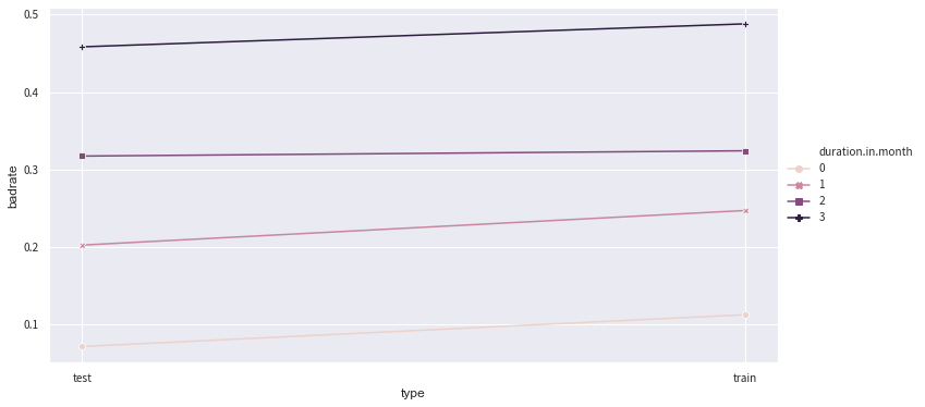
[11]:
# Assume we want to combine bin #1 and #2...
adj_bin = {'duration.in.month': [9, 18,33]}
c2.set_rules(adj_bin)

temp_data = c2.transform(data_[['duration.in.month','creditability','type']])
badrate_plot(temp_data, target = 'creditability', x = 'type', by = 'duration.in.month')

adj_bin = {'duration.in.month': [9, 18,33],'foreign.worker': [['no'], ['yes']]}
# therefore use this
[12]:
# Step 5: WOE transform with adjusted bins
combiner.set_rules(adj_bin)

binned_data = combiner.transform(selected_data)

transer = toad.transform.WOETransformer()
data_tr_woe = transer.fit_transform(binned_data, binned_data['creditability'], exclude=['creditability','type'])
data_ts_woe = transer.transform(combiner.transform(selected_test))
[13]:
binned_data.head(3) # the values are transformed into "index + bin" format
[13]:
| status.of.existing.checking.account | duration.in.month | credit.history | purpose | credit.amount | savings.account.and.bonds | present.employment.since | personal.status.and.sex | other.debtors.or.guarantors | property | age.in.years | other.installment.plans | housing | foreign.worker | creditability | type | |
|---|---|---|---|---|---|---|---|---|---|---|---|---|---|---|---|---|
| 569 | 3 | 3 | 1 | 1 | 2 | 3 | 2 | 2 | 0 | 2 | 2 | 0 | 0 | 1 | 1 | train |
| 574 | 2 | 1 | 1 | 1 | 0 | 3 | 1 | 1 | 0 | 2 | 1 | 0 | 0 | 1 | 0 | train |
| 993 | 3 | 3 | 1 | 2 | 2 | 3 | 4 | 1 | 0 | 1 | 2 | 0 | 0 | 1 | 0 | train |
III. Model selection
- toad.selection.stepwise(): this function performs feature selection (or model selection formally) with forward / backward / both-way stepwise. The function uses AIC / BIC as selection criterion.
[14]:
final_data = toad.selection.stepwise(data_tr_woe.drop('type',axis=1),target = 'creditability',direction = 'both', criterion = 'aic')

final_test = data_ts_woe[final_data.columns]
print(final_data.shape)
print(final_data.columns) # As shown, 15 features are down to 10 after both-way stepwise
(750, 10)
Index(['status.of.existing.checking.account', 'duration.in.month',
       'credit.history', 'purpose', 'age.in.years', 'other.installment.plans',
       'property', 'personal.status.and.sex', 'other.debtors.or.guarantors',
       'creditability'],
      dtype='object')
//anaconda3/lib/python3.7/site-packages/statsmodels/base/model.py:1294: RuntimeWarning: invalid value encountered in true_divide
  return self.params / self.bse
//anaconda3/lib/python3.7/site-packages/scipy/stats/_distn_infrastructure.py:877: RuntimeWarning: invalid value encountered in greater
  return (self.a < x) & (x < self.b)
//anaconda3/lib/python3.7/site-packages/scipy/stats/_distn_infrastructure.py:877: RuntimeWarning: invalid value encountered in less
  return (self.a < x) & (x < self.b)
//anaconda3/lib/python3.7/site-packages/scipy/stats/_distn_infrastructure.py:1831: RuntimeWarning: invalid value encountered in less_equal
  cond2 = cond0 & (x <= self.a)
[15]:
# Now ready to model. Fit a lr.
Xtr = final_data.drop('creditability',axis=1)
Ytr = final_data['creditability']
Xts = final_test.drop('creditability',axis=1)
Yts = final_test['creditability']

lr = LogisticRegression()
lr.fit(Xtr, Ytr)
//anaconda3/lib/python3.7/site-packages/sklearn/linear_model/logistic.py:432: FutureWarning: Default solver will be changed to 'lbfgs' in 0.22. Specify a solver to silence this warning.
  FutureWarning)
[15]:
LogisticRegression(C=1.0, class_weight=None, dual=False, fit_intercept=True,
                   intercept_scaling=1, l1_ratio=None, max_iter=100,
                   multi_class='warn', n_jobs=None, penalty='l2',
                   random_state=None, solver='warn', tol=0.0001, verbose=0,
                   warm_start=False)
IV. Model evaluation and validation
- Common evaluation metrics: toad. metrics. KS, F1, AUC
[16]:
from toad.metrics import KS, F1, AUC

EYtr_proba = lr.predict_proba(Xtr)[:,1]
EYtr = lr.predict(Xtr)

print('Training error')
print('F1:', F1(EYtr_proba,Ytr))
print('KS:', KS(EYtr_proba,Ytr))
print('AUC:', AUC(EYtr_proba,Ytr))

EYts_proba = lr.predict_proba(Xts)[:,1]
EYts = lr.predict(Xts)

print('\nTest error')
print('F1:', F1(EYts_proba,Yts))
print('KS:', KS(EYts_proba,Yts))
print('AUC:', AUC(EYts_proba,Yts))
Training error
F1: 0.4556701030927835
KS: 0.4872853159929582
AUC: 0.8107664187464729

Test error
F1: 0.45079365079365086
KS: 0.4771302530763873
AUC: 0.7811314913706369
- toad.metrics.PSI(): return the PSI of each feature to detect data migration
[17]:
psi = toad.metrics.PSI(final_data,final_test)
psi.sort_values(0,ascending=False) # Further tune the unstable feature if any
[17]:
purpose                                0.053175
duration.in.month                      0.038424
age.in.years                           0.017464
property                               0.014331
credit.history                         0.012744
status.of.existing.checking.account    0.001251
personal.status.and.sex                0.001096
creditability                          0.000545
other.installment.plans                0.000047
other.debtors.or.guarantors            0.000000
dtype: float64
- toad.metrics.KS_bucket(predicted_proba, y_true, bucket=10, method = ‘quantile’): output the result table including bad_rate, KS etc.
[18]:
tr_bucket = toad.metrics.KS_bucket(EYtr_proba,Ytr,bucket=10,method='quantile')
tr_bucket
[18]:
| min | max | bads | goods | total | bad_rate | good_rate | odds | bad_prop | good_prop | cum_bads | cum_goods | cum_bads_prop | cum_goods_prop | ks | |
|---|---|---|---|---|---|---|---|---|---|---|---|---|---|---|---|
| 0 | 0.012857 | 0.052979 | 0 | 75 | 75 | 0.000000 | 1.000000 | 0.000000 | 0.000000 | 0.143403 | 0 | 75 | 0.000000 | 0.143403 | -0.143403 |
| 1 | 0.053378 | 0.094267 | 1 | 74 | 75 | 0.013333 | 0.986667 | 0.013514 | 0.004405 | 0.141491 | 1 | 149 | 0.004405 | 0.284895 | -0.280490 |
| 2 | 0.094706 | 0.129116 | 9 | 66 | 75 | 0.120000 | 0.880000 | 0.136364 | 0.039648 | 0.126195 | 10 | 215 | 0.044053 | 0.411090 | -0.367037 |
| 3 | 0.130818 | 0.173092 | 14 | 61 | 75 | 0.186667 | 0.813333 | 0.229508 | 0.061674 | 0.116635 | 24 | 276 | 0.105727 | 0.527725 | -0.421998 |
| 4 | 0.173933 | 0.241864 | 20 | 55 | 75 | 0.266667 | 0.733333 | 0.363636 | 0.088106 | 0.105163 | 44 | 331 | 0.193833 | 0.632887 | -0.439055 |
| 5 | 0.242644 | 0.324243 | 18 | 57 | 75 | 0.240000 | 0.760000 | 0.315789 | 0.079295 | 0.108987 | 62 | 388 | 0.273128 | 0.741874 | -0.468746 |
| 6 | 0.324983 | 0.422900 | 29 | 46 | 75 | 0.386667 | 0.613333 | 0.630435 | 0.127753 | 0.087954 | 91 | 434 | 0.400881 | 0.829828 | -0.428947 |
| 7 | 0.424597 | 0.529979 | 37 | 38 | 75 | 0.493333 | 0.506667 | 0.973684 | 0.162996 | 0.072658 | 128 | 472 | 0.563877 | 0.902486 | -0.338609 |
| 8 | 0.532320 | 0.649534 | 45 | 30 | 75 | 0.600000 | 0.400000 | 1.500000 | 0.198238 | 0.057361 | 173 | 502 | 0.762115 | 0.959847 | -0.197732 |
| 9 | 0.652615 | 0.921777 | 54 | 21 | 75 | 0.720000 | 0.280000 | 2.571429 | 0.237885 | 0.040153 | 227 | 523 | 1.000000 | 1.000000 | 0.000000 |
V. Scorecard transformation
Toad allows scorecard transformation from bins and convert probability of credit risk into scores accordingly. 1. toad.scorecard.ScoreCard():
1.1 ScoreCard().predict(X): output scores with original features. The function uses combiner and transer to bin the original feature to predict the risk scores.
[19]:
# Step 1: alignment for combiner and WOETransformer
transer.fit_transform(final_data,final_data['creditability'],exclude='creditability')

# Step 2: send combiner, transer, and model to scorecard
card = toad.scorecard.ScoreCard(combiner = combiner, transer = transer, model = lr)
card.export() # output the scorecard details
[19]:
{'status.of.existing.checking.account': {'no checking account': 145.5,
  '... >= 200 DM / salary assignments for at least 1 year': 98.01,
  '0 <= ... < 200 DM': 36.69,
  '... < 0 DM': 4.62},
 'duration.in.month': {'[-inf ~ 9)': 159.42,
  '[9 ~ 18)': 85.84,
  '[18 ~ 33)': 56.47,
  '[33 ~ inf)': 3.34},
 'credit.history': {'critical account/ other credits existing (not at this bank)': 97.33,
  'existing credits paid back duly till now': 61.67,
  'delay in paying off in the past': 52.58,
  'all credits at this bank paid back duly,no credits taken/ all credits paid back duly': 2.79},
 'purpose': {'domestic appliances,car (used),retraining': 140.7,
  'radio/television': 96.33,
  'furniture/equipment': 52.36,
  'repairs,business,car (new)': 42.25,
  'education,others': 5.55},
 'age.in.years': {'[-inf ~ 26)': 119.2,
  '[26 ~ 28)': 88.33,
  '[28 ~ 35)': 79.77,
  '[35 ~ 39)': 69.03,
  '[39 ~ 49)': 51.42,
  '[49 ~ inf)': 29.62},
 'other.installment.plans': {'none': 76.53, 'bank,stores': 16.83},
 'property': {'real estate': 96.25,
  'building society savings agreement/ life insurance': 61.28,
  'car or other, not in attribute Savings account/bonds': 56.62,
  'unknown / no property': 33.45},
 'personal.status.and.sex': {'male : married/widowed': 83.32,
  'male : single': 77.63,
  'female : divorced/separated/married': 41.74}}
[20]:
# Step 3: predict scores
pred_scores = card.predict(data_ts)
print('Sample scores:',pred_scores[:10])
print('Test KS: ',KS(pred_scores, data_ts['creditability']))
Sample scores: [691.85512232 376.40390218 642.23643223 549.8182956  528.58400131
 585.98431629 598.46669667 477.92206049 569.01975099 665.1492379 ]
Test KS:  0.3830972834919898
[ ]: